CPP Data Structure
- Circular buffer / Ring buffer (环形队列缓存)
- False sharing (伪共享)
- 平衡二叉树(AVL)
- B树
- B+树
- 红黑树
- Trie 树 (前缀树 / 字典树)
- 堆(数组实现)
Circular buffer / Ring buffer (环形队列缓存)
In computer science, a circular buffer, circular queue, cyclic buffer or ring buffer is a data structure that uses a single, fixed-size buffer as if it were connected end-to-end. This structure lends itself easily to buffering data streams. There were early circular buffer implementations in hardware.
Overview
A ring showing, conceptually, a circular buffer. This visually shows that the buffer has no real end and it can loop around the buffer. However, since memory is never physically created as a ring, a linear representation is generally used as is done below.
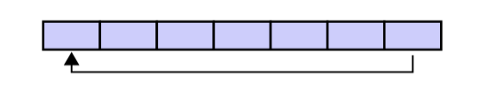
A circular buffer first starts out empty and has a set length. In the diagram below is a 7-element buffer:
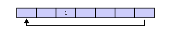
Assume that 1 is written in the center of a circular buffer (the exact starting location is not important in a circular buffer):
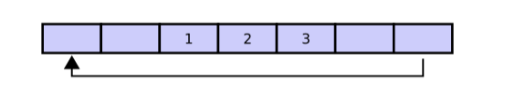
Then assume that two more elements are added to the circular buffer — 2 & 3 — which get put after 1:
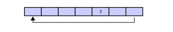
If two elements are removed, the two oldest values inside of the circular buffer would be removed. Circular buffers use FIFO (first in, first out) logic. In the example, 1 & 2 were the first to enter the circular buffer, they are the first to be removed, leaving 3 inside of the buffer.
If the buffer has 7 elements, then it is completely full:
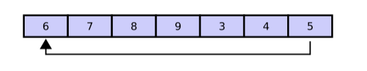
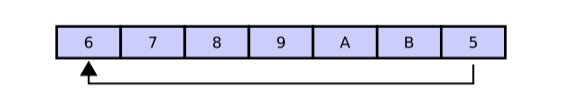
A property of the circular buffer is that when it is full and a subsequent write is performed, then it starts overwriting the oldest data. In the current example, two more elements — A & B — are added and they overwrite the 3 & 4:
Alternatively, the routines that manage the buffer could prevent overwriting the data and return an error or raise an exception. Whether or not data is overwritten is up to the semantics of the buffer routines or the application using the circular buffer.
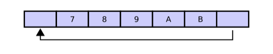
Finally, if two elements are now removed then what would be removed is not A & B, but 5 & 6 because 5 & 6 are now the oldest elements, yielding the buffer with:
False sharing (伪共享)
In computer science, false sharing is a performance-degrading usage pattern that can arise in systems with distributed, coherent caches at the size of the smallest resource block managed by the caching mechanism. When a system participant attempts to periodically access data that is not being altered by another party, but that data shares a cache block with data that is being altered, the caching protocol may force the first participant to reload the whole cache block despite a lack of logical necessity. The caching system is unaware of activity within this block and forces the first participant to bear the caching system overhead required by true shared access of a resource.
伪共享是计算机科学中一种会导致性能下降的使用模式。它主要发生在具有分布式、一致性缓存的系统(比如多核CPU)中,问题的关键粒度是缓存机制管理的最小资源块(通常是缓存行)。
在一个多核系统中,每个核心都有自己的缓存(比如L1、L2缓存),并且这些缓存通过某种协议(如 MESI)保持数据一致性。缓存从主内存加载数据不是一个个字节加载的,而是按固定大小的块(缓存行,Cache Line,常见大小如 64 字节)加载。
伪共享就是多个处理器核心频繁访问逻辑上独立但物理上位于同一个缓存行中的数据时,由于缓存一致性协议需要以整个缓存行为单位维护一致性,导致一个核心修改自己的数据会无效化另一个核心的缓存(即使后者访问的数据没变),迫使后者不必要地重新加载整个缓存行,从而造成严重的性能下降。它是由于缓存管理粒度(缓存行)与应用数据访问粒度不匹配引发的一种“误伤”现象。
实际应用的例子:SPSCQueue 优化 False sharing 问题的设计 https://github.com/rigtorp/SPSCQueue/blob/master/README.md
- 头尾指针隔离
head(读指针)和tail(写指针)被分别对齐到独立的缓存行(通常 64 字节)。- 实现方式:通过编译器指令(如
alignas(64))和显式填充(Padding)确保每个指针独占一个缓存行。 - 效果:生产者更新
tail时不会使消费者缓存中的head失效,反之亦然,消除核心间的无效化风暴。
- 缓冲区边界隔离
- 数据缓冲区(
slots)的起始和结束位置添加填充,使其与相邻内存隔离。 - 原因:避免其他变量(如堆分配器元数据)与缓冲区共享缓存行,防止外部操作引发伪共享。
- 数据缓冲区(
平衡二叉树(AVL)
在计算机科学中,AVL树(科学家的英文名,前苏联的数学家 Adelse-Velskil 和 Landis 在 1962 年提出的高度平衡的二叉树)是最早被发明的自平衡二叉查找树。在AVL树中,任一节点对应的两棵子树的最大高度差为1,因此它也被称为高度平衡树。查找、插入和删除在平均和最坏情况下的时间复杂度都是O(logN)。
平衡二叉树特点:
- 非叶子节点最多拥有两个子节点;
- 非叶子节值大于左边子节点、小于右边子节点;
- 树的左右两边的层级数相差不会大于1;
- 没有值相等重复的节点;
为什么要有平衡二叉树
二叉搜索树一定程度上可以提高搜索效率,但是当原序列有序时,例如序列 A = {1,2,3,4,5,6},构造二叉搜索树如下:
1
 \
  2
   \
    3
     \
      4
       \
        5
         \
          6
依据此序列构造的二叉搜索树为右斜树,同时二叉树退化成单链表,搜索效率降低为O(n)。二叉搜索树的查找效率取决于树的高度,因此保持树的高度最小,即可保证树的查找效率。若改为如下存储方式,查询只需要比较3次(查询效率提升一倍):
            3
         /      \
        2        5
       /        / \
      1        4   6
可以看出当节点数目一定,保持树的左右两端保持平衡,树的查找效率最高。这种左右子树的高度相差不超过 1 的树为平衡二叉查找树(简称,平衡二叉树)。
平衡因子
某节点的左子树与右子树的高度(深度)差即为该节点的平衡因子(BF,Balance Factor),平衡二叉树中不存在平衡因子大于 1 的节点。在一棵平衡二叉树中,节点的平衡因子只能取 0 、1 或者 -1 ,分别对应着左右子树等高,左子树比较高,右子树比较高。
节点定义
typedef struct AVLNode *Tree;

typedef int ElementType;

struct AVLNode{

    int depth;       // 深度,这里计算每个节点的深度,通过深度的比较可得出是否平衡

    Tree parent;     // 该节点的父节点

    ElementType val; // 节点值

    Tree lchild;

    Tree rchild;

    AVLNode(int val = 0) {
        parent = NULL;
        depth = 0;
        lchild = rchild = NULL;
        this->val = val;
    }
};
refer:
- https://zh.wikipedia.org/wiki/AVL%E6%A0%91
- https://zhuanlan.zhihu.com/p/56066942
B树
B树和平衡二叉树稍有不同的是B树属于多叉树又名平衡多路查找树(查找路径不只两个),数据库索引技术里大量使用者B树和B+树的数据结构。
特点:
B树相对于平衡二叉树的不同是,每个节点包含的关键字增多了,特别是在B树应用到数据库中的时候,数据库充分利用了磁盘块的原理(磁盘数据存储是采用块的形式存储的,每个块的大小为4K,每次IO进行数据读取时,同一个磁盘块的数据可以一次性读取出来)把节点大小限制和充分使用在磁盘快大小范围;把树的节点关键字增多后树的层级比原来的二叉树少了,减少数据查找的次数和复杂度。
A B-Tree is a specialized m-way tree designed to optimize data access, especially on disk-based storage systems. In a B-Tree of order m, each node can have up to m children and m-1 keys, allowing it to efficiently manage large datasets.
One of the standout features of a B-Tree is its ability to store a significant number of keys within a single node, including large key values. It significantly reduces the tree’s height, hence reducing costly disk operations. B Trees allow faster data retrieval and updates, making them an ideal choice for systems requiring efficient and scalable data management. By maintaining a balanced structure at all times, B-Trees deliver consistent and efficient performance for critical operations such as search, insertion, and deletion.
Properties of a B-Tree:
A B Tree of order m can be defined as an m-way search tree which satisfies the following properties:
- All leaf nodes of a B tree are at the same level, i.e. they have the same depth (height of the tree). (所有叶子节点都在相同的层级)
- The keys of each node of a B tree (in case of multiple keys), should be stored in the ascending order. (每个节点包含多个 key 以升序排列)
- In a B tree, all non-leaf nodes (except root node) should have at least
m/2children. (除了根节点,所有非叶子节点应该包含至少m/2个子节点) - All nodes (except root node) should have at least
m/2 - 1keys. (除了根节点,所有节点应该包含至少m/2 - 1个 key) - If the root node is a leaf node (only node in the tree), then it will have no children and will have at least one key. If the root node is a non-leaf node, then it will have at least 2 children and at least one key.
- A non-leaf node with
n-1key values should havennon NULL children.
Following is an example of a B-Tree of order 5.
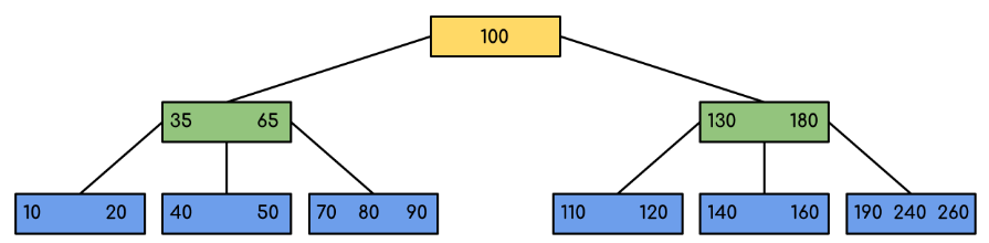
We can see in the above diagram that all the leaf nodes are at the same level and all non-leaf nodes have no empty sub-tree and have number of keys one less than the number of their children.
B+树
B+树是B树的一个升级版,相对于B树来说B+树更充分的利用了节点的空间,让查询速度更加稳定,其速度完全接近于二分法查找。
特点:
- B+树的层级更少:相较于B树B+树每个非叶子节点存储的关键字数更多,树的层级更少所以查询数据更快;
- B+树查询速度更稳定:B+树所有关键字数据地址都存在叶子节点上,所以每次查找的次数都相同所以查询速度要比B树更稳定;
- B+树天然具备排序功能:B+树所有的叶子节点数据构成了一个有序链表,在查询大小区间的数据时候更方便,数据紧密性很高,缓存的命中率也会比B树高。
- B+树全节点遍历更快:B+树遍历整棵树只需要遍历所有的叶子节点即可,而不需要像B树一样需要对每一层进行遍历,这有利于数据库做全表扫描。
红黑树
红黑树是一种自平衡二叉查找树,典型的用途是实现关联数组。红黑树的结构复杂,但它的操作有着良好的最坏情况运行时间,它可以在O(logN)时间内完成查找、插入和删除。
红黑树相对于AVL树来说,牺牲了部分平衡性以换取插入/删除操作时少量的旋转操作,整体来说性能要优于AVL树。
Trie 树 (前缀树 / 字典树)
Trie 树,是一个像查字典一样的树形结构,一般会选择字符串作为键 (key),并非像二叉搜索树那样直接保存到每一个树节点。在 Trie 树中,键会被打散分布于一条树链上。例如,用键集:{“romane”,”romanes”,”romanus”,”romulus”,”rubens”,”ruber”,”rubes”,”rubicon”,”rubicundus”,”rubric”},构建一棵传统 Trie 树:
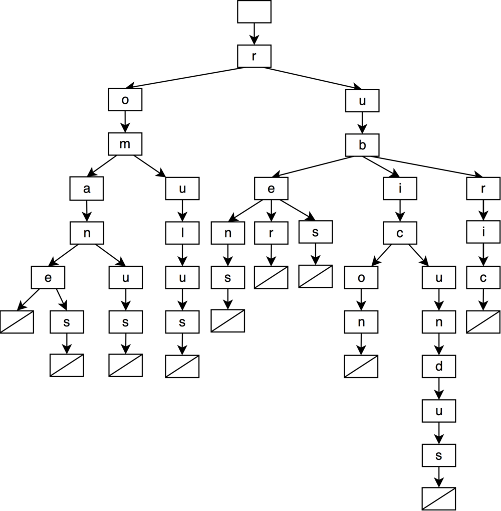
如图所示,从根节点开始,任选一条到叶子结点的树链,这条路径上的字符所组成的字符串对应了集合中的特定键,此树一共有 10 个叶子节点,分别对应 10 个键。图中的叶子结点是个哨兵,它不存储任何字符,只是单纯代表字符串的终止。
Trie 树最基础的应用就是,字符串的查找 —— 判断某个字符串是否在字典中。当需要查找某个字符串是否存在于 key 集时,只需要逐字符 match,层层递进,如果在遍历到最后一个字符时可以命中叶子节点,那么就代表它存在,否则在中途中任何一步没能 match,就代表不存在。
正因为这一典型应用,Trie 树又叫字典树。实际上,除了判断字符串是否存在,还可以在这个基础上,利用 Trie 做词频统计。只需要在每个叶子节点的值域存储一个计数器即可。词频统计正是 Trie 的常见应用场景之一。
这样的结构就像是一棵 K 叉树,在检索字符串的过程中,途径每层都在做同一件事:判断当前的父节点是否存在待检索字符所对应的子节点,如果有就递归向下,没有就终止。可以发现,具有相同前缀的字符串,它们在树中会共享非叶子节点,相比于用哈希表去存储全量键集,Trie 得益于共享前缀的特性,体积的缩小肉眼可见。
哈希表当然可以完成判断字符串是否在字典中的任务,查询的时间复杂度是 O(1),这意味着它的查找很快,显然,这是用空间换来的。
相比于哈希表,Trie 的查询速度显然劣势,Trie 牺牲了时间去换取了大量的空间节省,它的时间复杂度是 O(len),其中 len 表示查询字符串的长度。
堆(数组实现)
堆的定义
堆是一种非线性结构,可以把堆看作一个数组,也可以被看作一个完全二叉树,堆其实就是利用完全二叉树的结构来维护的一维数组。按照堆的特点可以把堆分为:
- 大顶堆:每个结点的值都大于或等于其左右孩子结点的值。
- 小顶堆:每个结点的值都小于或等于其左右孩子结点的值。
堆的这种特性非常的有用,常常被当做优先队列使用,因为可以快速访问到“最重要”的元素
堆的数组实现
- arr[0]为根节点
- 大顶堆:arr[i] >= arr[2i+1] && arr[i] >= arr[2i+2]
- 小顶堆:arr[i] <= arr[2i+1] && arr[i] <= arr[2i+2]
例如:大顶堆,用数组arr表示为:10 9 8 7 6 4 5 1 3
            10
         /      \
        9        8
       / \      / \
      7   6    4   5
     / \
    1   3
堆和普通树的区别
- 内存占用。普通树的实现方式空间浪费比较大
- 平衡。在堆中不需要整棵树都是有序的,只需要满足堆的属性即可,所以在堆中平衡不是问题,因此堆中数据的组织方式可以保证O(nlog2n) 的性能;而普通树需要在“平衡”的情况下,其时间复杂度才能达到O(nlog2n)
- 搜索。在二叉树中搜索会很快,但是在堆中搜索会很慢。在堆中搜索不是第一优先级,因为使用堆的目的是将最大(或者最小)的节点放在最前面,从而快速的进行相关插入、删除操作
堆排序的过程
算法思想:将待排序序列构造成一个大顶堆(生序排序),此时,整个序列的最大值就是堆顶的根节点。将根节点与末尾元素进行交换,此时末尾就为最大值。然后将剩余n-1个元素重新构造成一个堆,这样会得到n个元素的次小值。如此反复执行,便能得到一个有序序列了。注意,建立大顶堆时是从最后一个非叶子节点开始从下往上调整的。
例如:
int a[6] = {7, 3, 8, 5, 1, 2};
对应的二叉树为:
          7
       /      \
      3        8
     / \      /
    5   1    2
通过构建大顶堆,实现升序排序。(同理,小顶堆对应降序排序):
step 1: 先找到最后一个非叶子节点 len(arr) / 2 - 1 = 6 / 2 - 1 = 2,即 a[2],如果 a[2] 小于 其左右子节点的值则交换,8 > 2 不需要交换
          7
       /      \
      3        **8(起始节点)**
     / \      /
    5   1    2
step 2: 继续找到下一个非叶子节点(即当前坐标 - 1)a[1],判断 a[1] < 左子节点的值,则交换值。交换后大于右子节点的值,则不交换
          7
       /      \
      5        8
     / \      /
    3   1    2
step 3: 继续找到下一个非叶子节点 (即当前坐标 - 1)a[0],判断 a[0] > 左子节点的值,则不交换,a[0] < 右子节点的值,则交换值
          8
       /      \
      5        7
     / \      /
    3   1    2
step 4: 检查调整后的子树,是否满足大顶堆性质,如果不满足则继续调整
step 5: 若大顶堆已构建完成,然后交换根节点与最后一个元素,此时最大的元素已经归位,然后对剩下的元素重复上面的操作
          2
       /      \
      5        7
     / \      /
    3   1    **8(已归位)**
step 6: 最终可以得到升序序列:1 2 3 5 7 8
          1
       /      \
      2        3
     / \      /
    5   7    8
堆排序实现代码
#include <iostream>
#include <vector>

// 这里实现并非调整到严格意义上的大顶堆,只是保证根节点为最大值
// 若要构建完整的大顶堆,则需要在交换节点后递归调整子树
void build_max_heap(std::vector<int> &a, int len)
{
    for (int i = len / 2 - 1; i >= 0; --i) {
        if ( (2 * i + 1) < len && a[i] < a[2 * i + 1] ) {
            // 最后一个非叶子节点 < 左子节点
            std::swap(a[i], a[2 * i + 1]);
        }

        if ( (2 * i + 2) < len && a[i] < a[2 * i + 2] ) {
            // 最后一个非叶子节点 < 右子节点
            std::swap(a[i], a[2 * i + 2]);
        }
    }
}

int main()
{
    std::vector<int> a = {7, 3, 2, 5, 6, 0, -1, 8, 8};
    size_t len = a.size();

    for (size_t i = len; i > 0; --i) {
        build_max_heap(a, static_cast<int>(i));

        // 输出当前迭代结果
        std::cout << "\n" << i << " ------------\n";
        for (auto &i : a) {
            std::cout << i << " ";
        }


        std::swap(a[0], a[i - 1]);// 交换大顶堆定一个元素与最后一个元素, 最后一个元素作为最大值归位
    }

    std::cout << "\nres:\n";
    for (auto &i : a) {
        std::cout << i << " ";
    }

    return 0;
}
/*
9 ------------
8 7 2 3 6 0 -1 5 8
8 ------------
8 7 2 5 6 0 -1 3 8
7 ------------
7 3 2 5 6 0 -1 8 8
6 ------------
6 -1 2 3 5 0 7 8 8
5 ------------
5 0 2 -1 3 6 7 8 8
4 ------------
3 0 2 -1 5 6 7 8 8
3 ------------
2 -1 0 3 5 6 7 8 8
2 ------------
0 -1 2 3 5 6 7 8 8
1 ------------
-1 0 2 3 5 6 7 8 8
res:
-1 0 2 3 5 6 7 8 8
*/
注意,这里实现并非调整到严格意义上的大顶堆,只是保证根节点为最大值(但是,可以满足排序的需求)。
例如,初始状态为:
          7
       /      \
      3        2
     / \      / \
    5   6    0   -1
   / \
  8   8
第一轮build_max_heap后,结果为:(并不满足大顶堆)
          8
       /      \
      7        2
     / \      / \
    3   6    0   -1
   / \
  8   5
若要构建完整的大顶堆,则需要在交换节点后递归调整子树,调整代码如下:
#include <iostream>
#include <vector>

void build_max_heap(std::vector<int> &a, int len)
{
    for (int i = len / 2 - 1; i >= 0; --i) {
        if ( (2 * i + 1) < len && a[i] < a[2 * i + 1] ) {
            // 最后一个非叶子节点 < 左子节点
            std::swap(a[i], a[2 * i + 1]);

            // 递归调整左子树
            if ((2 * (2 * i + 1) + 1 < len && a[2 * i + 1] < a[2 * (2 * i + 1) + 1])
               || (2 * (2 * i + 1) + 2 < len && a[2 * i + 1] < a[2 * (2 * i + 1) + 2])) {
                build_max_heap(a, len);
            }
        }

        if ( (2 * i + 2) < len && a[i] < a[2 * i + 2] ) {
            // 最后一个非叶子节点 < 右子节点
            std::swap(a[i], a[2 * i + 2]);

            // 递归调整右子树
            if ((2 * (2 * i + 2) + 1 < len && a[2 * i + 2] < a[2 * (2 * i + 2) + 1])
               || (2 * (2 * i + 2) + 2 < len && a[2 * i + 2] < a[2 * (2 * i + 2) + 2])) {
                build_max_heap(a, len);
            }
        }
    }
}

int main()
{
    std::vector<int> a = {7, 3, 2, 5, 6, 0, -1, 8, 8};
    size_t len = a.size();

    for (size_t i = len; i > 0; --i) {
        build_max_heap(a, static_cast<int>(i));

        // 输出当前迭代结果
        std::cout << "\n" << i << " ------------\n";
        for (auto &i : a) {
            std::cout << i << " ";
        }


        std::swap(a[0], a[i - 1]);// 交换大顶堆定一个元素与最后一个元素, 最后一个元素作为最大值归位
    }

    std::cout << "\nres:\n";
    for (auto &i : a) {
        std::cout << i << " ";
    }

    return 0;
}
/*
9 ------------
8 8 2 7 6 0 -1 3 5
8 ------------
8 7 2 5 6 0 -1 3 8
7 ------------
7 6 2 3 5 0 -1 8 8
6 ------------
6 5 2 -1 3 0 7 8 8
5 ------------
5 3 2 -1 0 6 7 8 8
4 ------------
3 0 2 -1 5 6 7 8 8
3 ------------
2 -1 0 3 5 6 7 8 8
2 ------------
0 -1 2 3 5 6 7 8 8
1 ------------
-1 0 2 3 5 6 7 8 8
res:
-1 0 2 3 5 6 7 8 8
*/
第一轮build_max_heap后,结果为:(满足大顶堆)
          8
       /      \
      8        2
     / \      / \
    7   6    0   -1
   / \
  3   5
堆的应用
例如:10亿数据中取最大的100个数据
思路:假设,N = 10亿,M = 100,则先取出前M个数,维护一个M个数的最小堆,遍历一遍剩余的元素,在此过程中维护小顶堆就可以了。具体步骤如下:
- 取前
M个元素,建立一个小顶堆。保持一个小顶堆得性质的步骤,运行时间为O(logM)。因此,建立一个小顶堆运行时间为:M \* O(logM)。 - 顺序读取后续元素,直到结束。每次读取一个元素,如果该元素比堆顶元素小直接丢弃;如果大于堆顶元素,则用该元素替换堆顶元素,然后保持最小堆性质。最坏情况是每次都需要替换掉堆顶的最小元素,因此需要维护堆的代价为
(N - M) \* O(logM)。最后这个堆中的元素就是前最大的100个。
refer:
- https://www.cnblogs.com/lanhaicode/p/10546257.html